par Raymond Koch, physicien

This paper is the transcript of my talk given at the European Physical Society Energy Group Meeting on 14/05/2024 in Cadarache (ITER).

Introduction. The present work is my attempt to make sense of what we are seeing and hearing in the press, in the media, in journals, in official statements from governments, scientific or activist groups and even from people around us about Climate. Trying also to understand why climate considerations are constraining if not ruling decisions on energy, mobility, social organization, and how they impact moral judgment. My point of view is that of a physicist, and this is the way I address the question below.

Evaluating the benefits

The fundamental law of global warming. The main feature of the climate turmoil is the alarm spread across the population that mankind’s emissions of carbon dioxide have deeply affected the earth climate, rocking it to a disrupted state, lethal for mankind if urgent drastic measures are not taken. This disrupted state is the consequence of a process named « global warming« . Global warming would be due to anthropic emissions, mainly of CO₂. Global warming causes another process defined as « climate change« . Climate change is a complete and closed process, an entity in itself that requires no further definition. It is a consequence of Global warming and as such possibly due to mankind’s activity. Climate change causes changes (plural) in climate and in weather, notably extreme meteorological events. Richard Lindzen explains (1) very well how the fear from climate change has replaced the fear of global warming in official climate discourses, because the latter (one or two °C increase over a century) was not visible enough on a day-to-day scale while meteorological catastrophes regularly happen somewhere in the world, can be shown worldwide on TV and can easily (rightly or wrongly) be attributed to climate change (Implicit: – caused by global warming caused by CO₂ emissions).

In order to estimate the benefits for climate to be expected from the Net-Zero program of the European Institutions, we need to understand the relation between the first two terms of the causal chain: CO₂ emissions and global warming. The nature of this relation is easily found in a picture, widely wielded as an alarm flag in the press and media, that shows the near-linear relationship between CO₂ increases and « temperature » increases, as shown in Fig.1. This figure

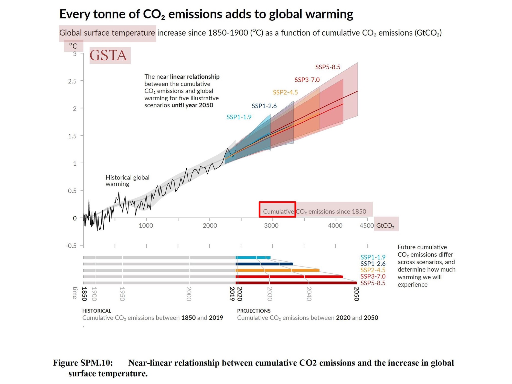
is extracted from the Summary for policy makers from the AR6 Group 1 report (2) of the IPCC, easily available. The comment about this picture is usually that it shows without any doubt how the world moves to complete overheating (2-2.5°C) and hence destruction if mankind does not stop immediately CO₂ emissions in the atmosphere. Fitting a straight line through this data, IPCC deduce a fundamental relation between CO₂ emissions and global warming:

[AR6 SPM-p.28 D.1.1] Each 1000 GtCO₂ of cumulative CO₂ emissions is assessed to likely cause a 0.27 °C to 0.63 °C increase in global surface temperature with a best estimate of 0.45 °C.

This establishes a fundamental relation between CO₂ emissions and temperature anomaly increases, in a simplified form :

1 cumulative TtCO2 ⟶ +0.45°C

It is important to note that this relation is based on « cumulative » emissions. Contrary to what one could think, in IPCC jargon, cumulative emissions are not the total amount of CO₂ that has been sent into the atmosphere due to human activities over a given period but only the part of it that remains in the atmosphere (3). The ratio of the two is called the airborne fraction. This quantity is not known very precisely, but following IPCC (4), it was around 44% for the last 60 years. This allows us to convert the above fundamental relation into what I shall call

and here 1 TtCO₂ is the quantity of CO₂ injected in the atmosphere by anthropic activities. With this relation, the benefit of a successful Net Zero plan in terms of a reduction in global warming can be evaluated.

The benefits of realizing the Net Zero plan are computed in Fig.2 (5).

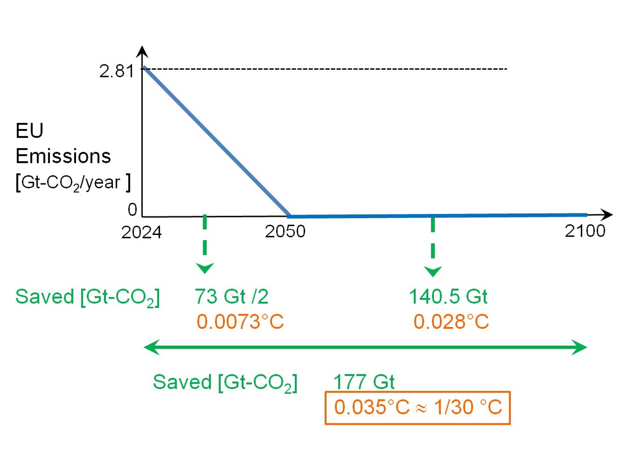
Fig.2 shows that in total from now to 2100 the Net Zero plan allows a reduction of 177 GTCO₂ as compared to a no-reduction strategy. This number is easily converted to a reduction of the an- thropogenic temperature increase using the fundamental law of global warming: 0.177 Tt CO₂ → 0.177×0.2°C=3.54×10⁻² °C. The avoided overheating is about one thirtieth of a degree centigrade.

The costs of Net Zero are according to Reuters (6) $1.6 trillion per year of investments, from now to 2050, to meet its net zero emissions target. As the EU Gross National product is estimated $19.35 trillion in 2024 (7), this represents some 7.5% of the GNP every year. The conclusions of this small exercise are straightforward:

Why did our leaders impose the Net Zero scheme? From the above, it is clear to any one believing in the AR6 IPCC summary for deciders and able to make a rule of three, that reaching the Net Zero holy grail will not at all save the planet. At first sight, it is strange that no one, in the large crowd of deciders and their assistants, had the idea to make the exercise of estimating the benefits of regulations that will completely revolutionize electrical power production, mobility, housing, food availability and so many other aspects of our society. The explanation resides in an age-old spontaneous mechanism of auto-polarization of society called ideology.

The new ideology is CLIMATISM. I cannot do better here than recommend the excellent book of Mike Hulme entitled Climate change isn’t everything (8) that precisely addresses this question of why the society and leaders engage in logically absurd, and sometimes insanely destructive, behavior and how Climatism polarizes society in a similar way, without, fortunately, having like former …isms, achieved its full maturity.

Climatism, like all totalizing ideologies contains the alpha and omega of knowledge of origin and fate of our universe, defines our moral principles and dictates rigidly all rules for behaving. It is a multi-millenia-old type of spontaneous social organization, which, this time,

• Is based on a major symbol, the global temperature that is the sign of everything: Eden climate at 0°C, catastrophe at +1.5°C and apocalypse at +2°C (9).

• Has its noble cause that prevails over other consideration: stop warming.

• Has as moral law indicator, the amount of CO₂ emissions (carbon footprint).

It holds all needed pseudo-rational justifications of leadership decisions. In this frame, the question of costs and benefits is secondary. What is important is to perform Grand, visible Noble gestures, in complete symbiosis with the faithful majority. Cost is not important because everything is secondary in the face of the saint objective and, actually, the more costly it is the more serious and determined the action looks. Estimating benefits is also unimportant, what counts is action. The more profound the implied changes to the society, the more conformal it is to ideology.

Climatism is the basis of political decisions. Like most previous …-isms, it is supported by a good fraction of the intellectual elite and scientific institutions. It is consensual. It cannot stand diverging opinions: there is only one truth and it is unassailable. For the climate ideology, the bible or party foundational text is the last IPCC report. That it is read by very few people (and essentially by no one in extenso) is not important because it is interpreted and taught by the climate priesthood. It has its prophets.

Because this ideology is constraining so much our freedom and attempting to replace an assumed old rogue and destructive social organization by a new one that saves the planet, it is important to dig a bit in the grounds on which the consensus rests.

Examining scientific foundations

Back to the settled science.  The observational basis of the fundamental law of global warming is Fig.1 discussed above. This figure shows that over a wide range of cumulative emissions (0 to 4.5 TtCO₂ , i.e. the double of the present value) one can confidently fit a straight line in the data. However, as a demonstration of the linearity it is definitely misleading because only the left part of the plot is actual observational data. The right part is made only from projections by climate codes, i.e. speculations. Restricting the cumulative emissions domain to

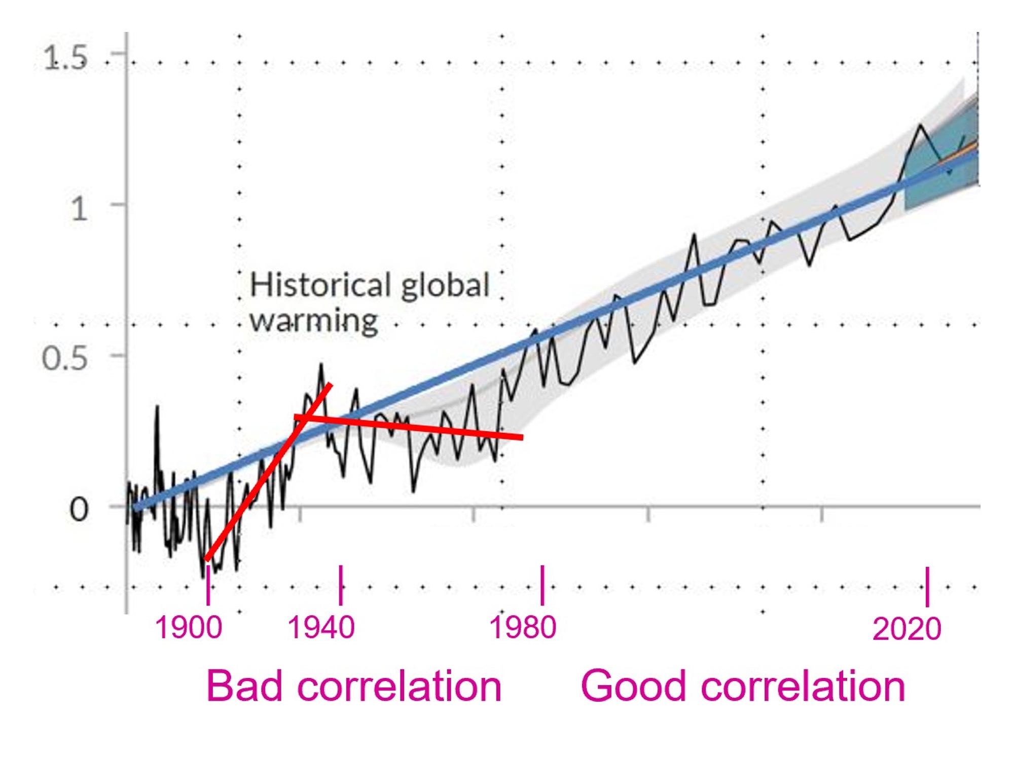
the observational range, we get Fig.3. The correlation is imperfect. There are two periods in which the observations notably diverge from the fundamental law. In between 1920 and 1940 the temperature increase is faster than predicted by the law while between 1940 and 1980 the temperature is nearly constant if not slightly decreasing. So, the linearity of the fundamental law rests on a short observational period of only some 45 years, from 1980 to presently. But this is its slightest flaw.

Correlation is not causality. It is not necessary to be clued up in statistics to guess that if you have two time-series that are moderately increasing and that you plot one versus the other and arrange scales to get the data around the diagonal, the plot that results will show some kind of near-linearity :

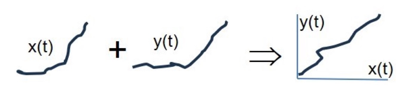
A real-world example of this can be found in a paper by Jamal Munshi (10). He takes as the two time-series the logarithm of the CO₂ concentration (because the radiative forcing by CO₂ increases only logarithmically with concentration) and the number of homicides in England and Wales in the period 1898-2003. The plot of homicide versus concentration is shown in Fig.4. The near-linear correlation is impossible to miss. Putting it in numbers and taking it seriously (as a parody) one can deduce a fundamental law causally linking CO₂ concentrations and homi- cides:

Each doubling of atmospheric CO2 causes 1.7 thousand of additional annual homicides in England and Wales.

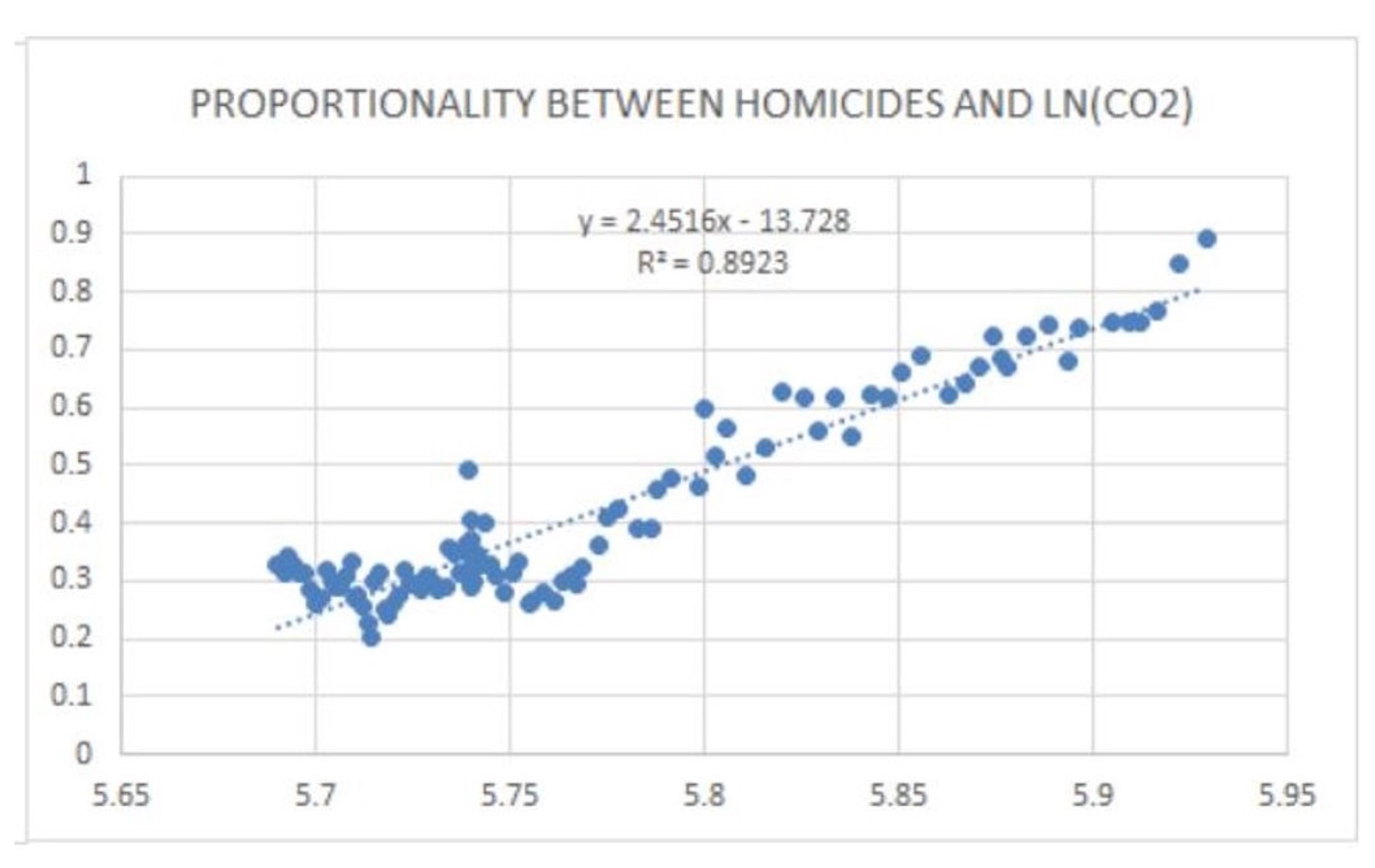
The paper further discusses the statistical methodologies that are to be followed before con- cluding that a real correlation between two time series exists and, incidentally, notes ‘This work demonstrates spurious proportionalities in time series data that may yield climate sensitivities that have no interpretation.’

This little discussion about the uncertainty of the correlation/causality between variations in CO₂ atmospheric concentrations and those of the Global Surface Temperature Anomaly (GSTA) requires us to come back to the exact nature of the GSTA. Here I shall focus on the physical meaning of a temperature average. To do that, let us first go back to good old 19th century thermodynamics.

An average of temperatures has generally speaking no physical meaning.  Thermodynamics distinguishes two main types of variables characterizing properties of physical systems: extensive and intensive variables. Examples of extensive variables are volume, mass, energy, number of particles. Pressure, density, temperature, are examples of intensive variables. Thermodynamics forbids adding up intensive variables (hence also, computing averages of these variables). If a system is composed of subsystems, the magnitude of the extensive variable for the whole system is the sum of its magnitudes in subsystems. If a system is composed of several volumes, the volume of the system is the sum of the volumes of the subsystems. Not so for intensive variables. Consider a car with a thermal engine. This is a physical system composed of several volumes (here assumed water proof): the interior cabin, that of tires, the inside of cylinders. One can add-up these volumes and get the total volume of water we would need to fill in these voids. Not the same for the intensive quantity ‘pressure’. If we add-up the cabin pressure, the tire pressures, the pressures inside cylinders, we get a total pressure that obviously has no meaning (especially if the engine is running). The resulting pressure cannot be measured anywhere. Dividing by the number of different volumes gives an average pressure per volume that has equally no meaning. Here the difference between extensive (volume) and intensive (pressure) quantities is intuitively clear. Pressure is not the amount of something. But what about temperature? This is less intuitive because we tend to confuse the temperature with an amount of heat. To clarify the question, I decided to do some ‘kindergarten’ physics to help intuition.

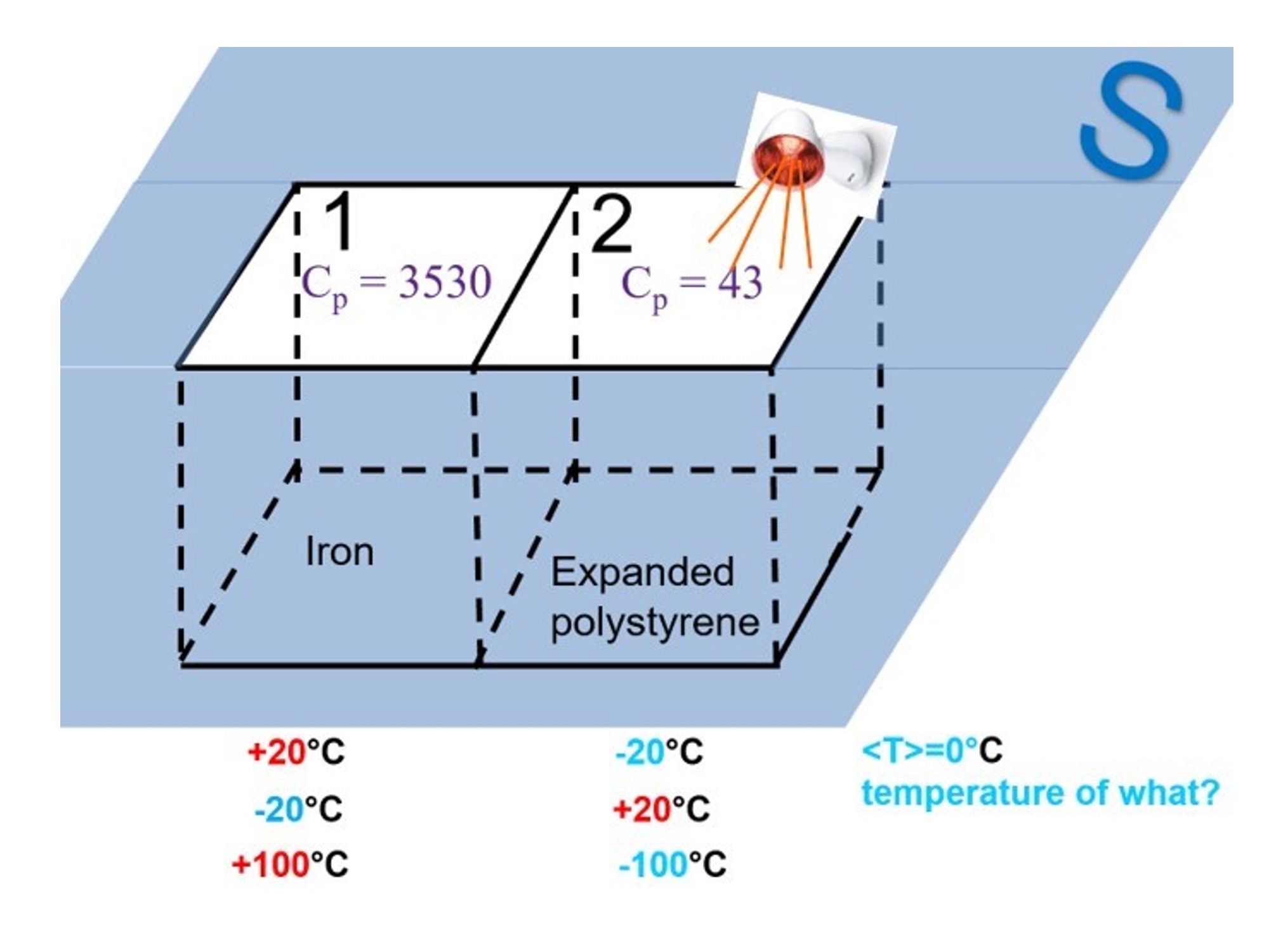
Consider Fig.5 and, for the time being let us forget about the infrared lamp above cube 2 and the different annotations, which will be introduced later on. Assume that at the initial instant the iron cube has been brought at +20°C and the polystyrene one at -20°C. Now, let us compute the average temperature that we will consider as the parameter that completely describes the system. It is < T >= (T₁ + T₂)/2 =(+20-20)/2 =0°C. It is actually a temperature of nothing in the system. Notice also that the same average < T > = 0°C can be obtained for an infinity of different temperature distributions, two examples being shown in the picture. As a parameter determining completely the thermal state of the two-cube system, it is particularly ineffective. Further, even the simple inversion (+20,-20) → (-20,+20) leads to a completely different thermal energy content and distribution because of the very different heat capacities (C_p) of iron and polystyrene.

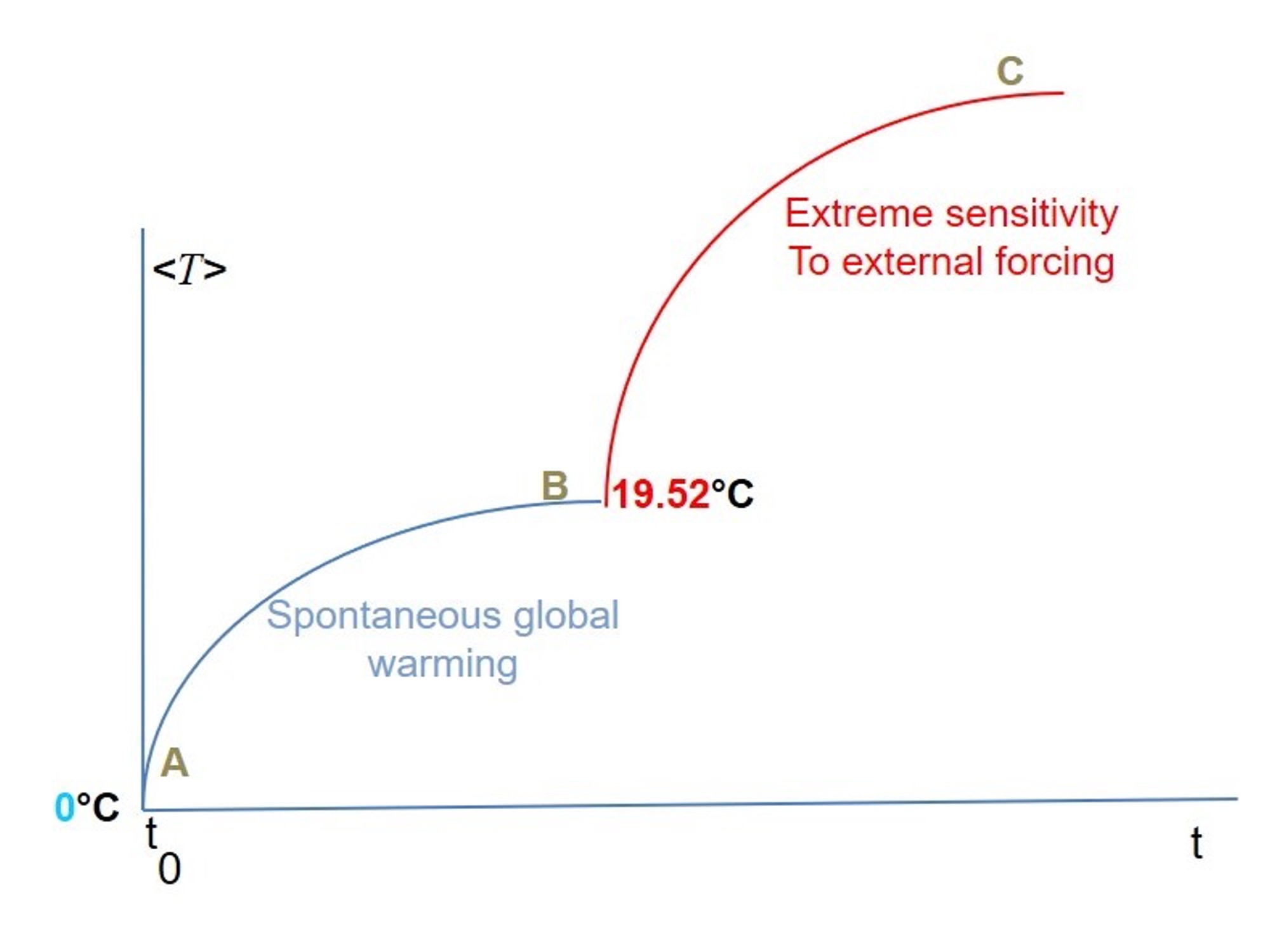
Now, for climate considerations we are interested in what the average temperature will tell us about the evolution of the system. Let us start again with the initial state (T₁=+20°C, T₂=- 20°C). If we let the system equilibrating, thermal energy will be transferred by conduction from 1 to 2, T₁ decreasing and T₂ increasing. For the average temperature, this is shown as the blue curve A-B in Fig.6. This is a purely internal process, with no external energy input to the system. At the end point B, the system has reached equilibrium T₁ + ∆T₁ = T₂ + ∆T₂. The total energy has been conserved C_p1∆T₁ + C_p2∆T₂ = 0 and this gives as equilibrium temperature 19.52°C. But the evolution of the average temperature tells us a quite different story if we consider <T> to be the ‘global temperature’ of the system. It tells that the total system has considerably increased its thermal energy (warmed up from 0°C to 19.52°C) without external input of energy: it has exhibited spontaneous global warming!

Above, we have considered volume averages. The situation is even worse if we attribute to the ‘surface average‘ (like for the GSTA) the potential of fully describing the state of the system. Indeed let us now (after having reached equilibrium point B) switch on the infrared lamp above surface 2 (Fig.5). Because polystyrene has very bad thermal conductivity and very low heat capacity the infrared power flux from the lamp will very quickly and strongly heat up a surface layer therefore raising quickly and considerably the value of the average surface temperature, even though the total heat content of the system has only slightly increased. Trusting the aver- age surface temperature therefore gives the impression that the system is extremely sensitive to external forcing. A wrong impression.

Can this happen in the climate system? Yes. The standard picture of global warming is that

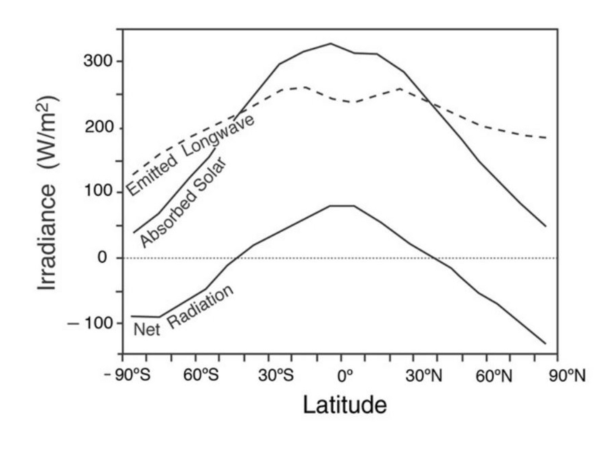
if the CO₂ concentration increases, it leads to a nearly uniform infrared radiative forcing (power flux to the surface) that will everywhere slightly increase, uniformly, the ground temperature, restoring the radiative balance. This picture rests on the implicit assumption (as strongly sug- gested by simple 1D climate models) (11) that the planet is in local radiative equilibrium, the sun and infrared power coming to the ground being everywhere balanced by outward infrared radiation. This is not the case, and this fact is well-known (12). Fig.7, and more precise distributions (13) show that the inter-tropical zone receives from the sun about 30% more power than what is sent back to space in the infrared. But globally the earth must be in radiative balance. And, indeed, conversely high latitudes radiate away more power than what they receive from the sun and the atmosphere above. So, some one-third of the global radiative balance of earth is operated through meridional power flows, i.e. convection in atmosphere and oceans, including transport of water and latent heat in clouds, of salinity in waters and other processes. Assume there is a slight change in these internal power flows; like in our two-cubes example, this can very well lead to unexplained spontaneous global warming (14), or cooling, observed in the global temperature.

Confronting the past

The return to the pre-industrial climate Eden. The Climatism fundamental moral command, grounded in physical science is stated by IPCC in AR6 :

[AR6 SPM-p.27 D.1] From a physical science perspective, limiting human-induced global warming to a specific level requires limiting cumulative CO₂ emissions, reaching at least net zero in CO₂ emissions, along with strong reductions in other greenhouse gas emissions.

How could anyone disobey an order dictated by physical science? This command is a clear statement that a return to the climate Eden climate is an absolute necessity. But that cannot be proven by a hard science, physics, because the concept of necessity or even desirability is not a concept of science but a concept of the social and political domains. Is going back to the pre-industrial climate really so desirable?

The question has been discussed by Roger Pielke Jr on his website (15), based on the book of Mike Davis (16). Here is a list of some main events in the period 1850-1900:

• The period starts with 50 million people deaths in the mid-1870s related to extreme weather and climate –That was about 4% of global population of the time. Related to that, a very strong El Niño event took place in 1877 and 1878.

• This was followed by many other extreme events with impacts well beyond those of recent times, such as the Great Midwest Wildfires of 1871 (2,400 deaths), the 1872 Baltic Sea flood, a 1875 Midwestern U.S. locust swarm of an estimated 12.5 trillion locusts, the 1878 China typhoon that killed as many as 100,000 people, and the U.S. experienced 6 land- falling major hurricanes in the 1870s, compared to just 3 in the 2010s.

• This ends in 1900 with, according to Wikipedia (17), the deadliest natural disaster in United States history, the Great Galveston hurricane (8,000 deaths). For comparison, Hurricane Katrina in 2005 caused 1,836 fatalities.

Eden climate? Really? I cannot have a better conclusion than Roger Pielke Jr.:

That notion that the period 1850 to 1900 was somehow safer or less extreme in terms of climate variations and impacts is simply false.

Is going straight to net-zero the optimal path? Ideologies frequently opt for an ‘all-or- nothing’ dictatorial-type strategy that often is nonsensical for solving problems. Climatism holds that there are no benefits in having more CO₂ but this is actually not true. A higher concentration is favorable to plant growth and the pre-industrial value, around 280 ppm concentration, was a bit lowish. The presently higher concentration, around 420 ppm, has led to earth greening (18) and increased agricultural productivity with reduced water requirements. Press screams bloody murder at casualties from hot temperature extremes but having milder cold extremes, also a consequence of global warming, save proportionally many more lives.

Would it not be wiser to stabilize CO₂ emissions at a value that balances advantages and drawbacks? If concentrations result from a balance between emissions and absorption, the latter being characterized by a lifetime τ of CO₂ molecules in the atmosphere, the concentration C will obey an equation like dC/dt = S_A-(C-C₀)/t  with C₀ the pre-industrial concentration and S_A the anthropic emissions rate. In absence of the latter one recovers the pre-industrial equilibrium C = C₀ and if anthropic emissions are stabilized at the constant level S_A, this model predicts a new stationary concentration level C_eq = C₀ + τ S_A. Although picturesque, this model has no predictive power because it ignores the changes in the ocean and land sinks (or sources), caused by changes in CO₂ concentration and temperature (AR6, Box TS.5, p.79). There is also a considerable uncertainty in the decay time τ . Modeling the climate system evolution after an abrupt shutdown of emissions with 18 Earth System Models (MacDougall et al.[19]) gives a large spread in the results. Out of nine curves (fig.2 of the paper) showing the CO₂ evolution over 100 years after shut-off, six give a decay time around 30 years and the three others a substantially larger one. Not less puzzling, and contrary to the fundamental law of global warming, the drop of some 100 ppm of concentration over 100 years is not accompanied by any significant temperature decrease in the ensemble average of the runs. Alternative analyzes by Salby & Harde (20) assert that the decay time is much shorter, about one year, and that the variations in CO₂ concentration essentially follow from temperature variations and show that this model accounts for both seasonal oscillations and long-term variations seen in the Keeling curve (21). According to this paper the anthropogenic component in these variations represents not more than 4%.

So, where is the bedrock of the urgency for an abrupt and universal cut of all CO₂ emissions?

At the world scale, according to Roger Pielke Jr (22), ‘To achieve net-zero by 2050 requires reducing unabated fossil fuel consumption by ≈ 25 EJ per year, or the equivalent of retiring 2 fossil fuel power plants every day‘.

CO₂–temperature causality: paleoclimate records  According to the discussion above, the motivation for an urgent cut of CO₂ emissions is at least obscure and it raises the next question: should we not rotate fig.3 180° around the main diagonal and read it as showing the CO₂ concentration increase due to increase in global temperature? What is the actual foundational status of the fundamental global warming law? We have seen that the linear fit founding this law is in agreement with the observational data only over a short period of 45 years (fig.3). Does it hold for a wider time span?

The science of the past climate has made tremendous progress over the last half century, providing information about the climate millions of years ago, which is really remarkable. Unfortunately IPCC AR6 report is not very illuminating on this topic (see Box TS.2 | Paleoclimate p.45-46), focusing on the tentative demonstration of the accuracy of specific paleoclimate code simulations or of the assertion that ‘changes observed since the 1950s are unprecedented over decades to millennia’ (p.41). A very good account, extensive, precise and didactic, of the progress made in understanding past climate can be found in the book by J. Vinós (23). This section is based on a few striking excerpts of the book, centered on the present discussion on the CO₂ – temperature correlation/causality.

Cenozoic Global temperature and CO₂ concentration have varied considerably in the past. Our first figure on this topic, fig.8, shows what happened over the past sixty million years.

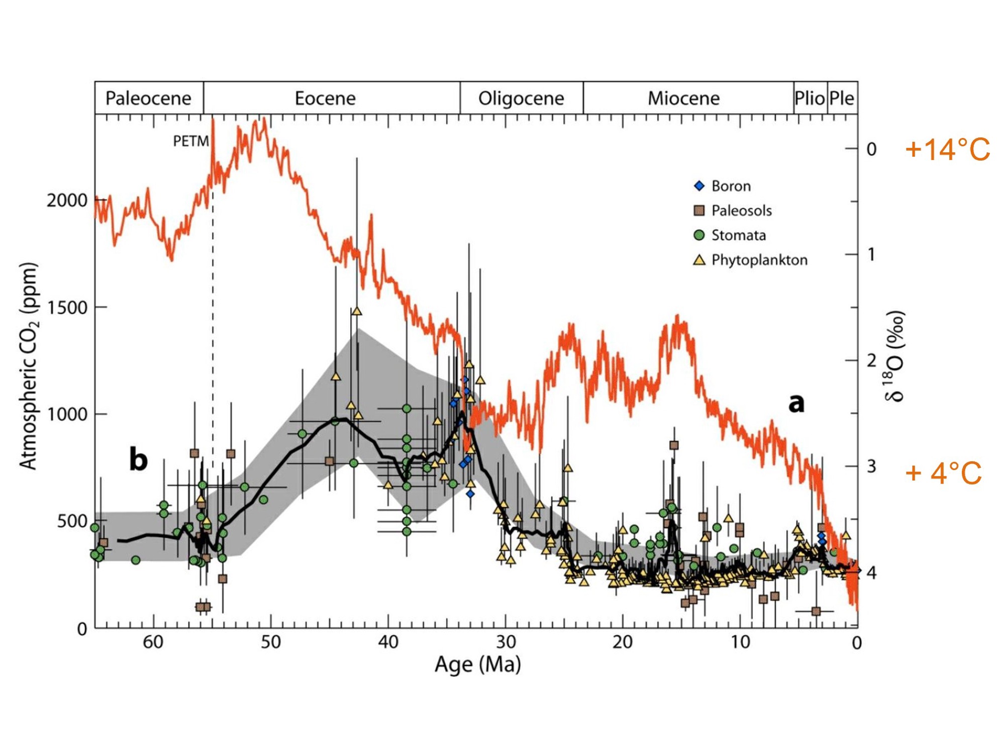
Two curves are shown. The red one is the curve of deviations of ¹⁸O concentrations. It is linearly and negatively correlated with the global temperatures such that the upside down δ¹⁸O curve is the temperature curve (24), with the equivalent temperatures indicated by the (+4°C, +14°C) points. One can observe that during most of this period temperatures were very high, with a peak during the Eocene thermal maximum 51 million years ago. The black curve is that of CO₂ concentration in the atmosphere. At the peak Eocene temperature, it is around 800 ppm. This corresponds to a mass of 6.3 TtCO₂ in the atmosphere (25). According to the Fundamental Law of Global Warming, this should have caused a warming of 2.8°C above pre-industrial value. Clearly this law is not universal enough to cover this past case. While there is good CO₂-Temperature correlation over the first quarter of Eocene (both are growing), the trends are opposite after the temperature peak, the CO₂ concentration continuing to grow while the temperature is falling down. Apart from this short period of co-evolution, which looks rather accidental, the two curves are uncorrelated.

60 million years of observation show no global correlation

Pleistocene The last million years are well-known for the -very roughly- hundred thousand years period oscillations between glaciations and much shorter interglacials, as shown in fig.9. We are presently in the last interglacial to the right of this picture.

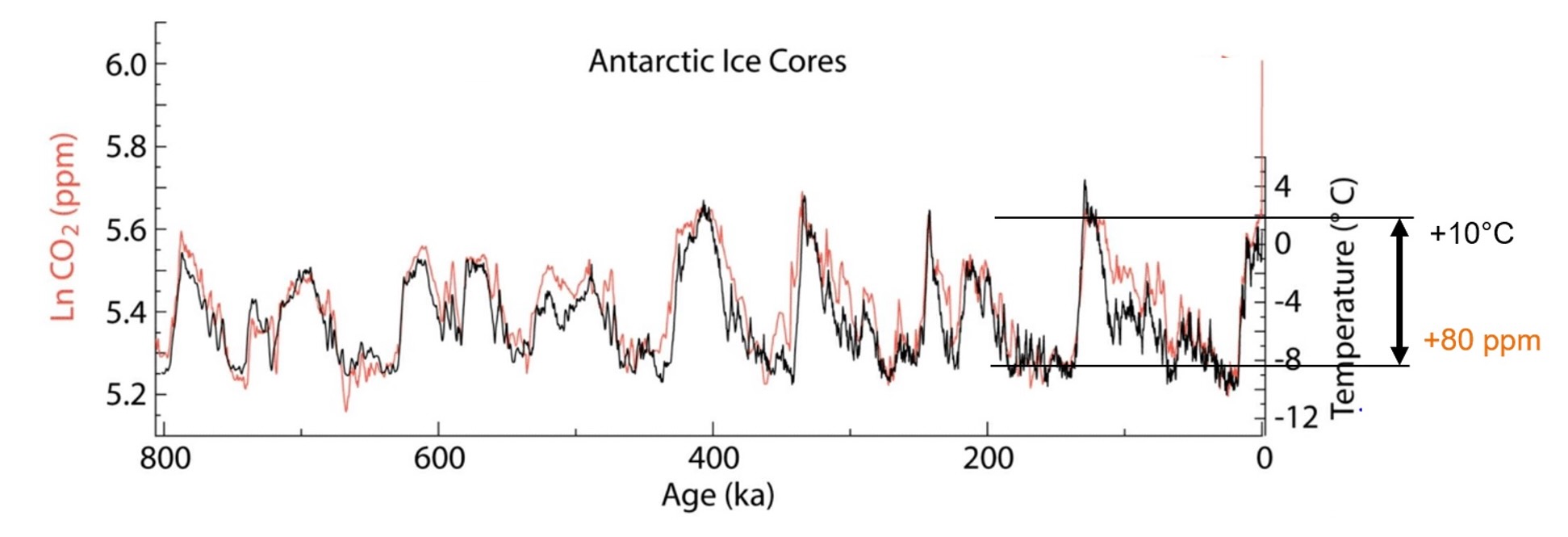
First, we can immediately observe the overall correlation between CO₂ and temperature variations. In a sense this is a confirmation of the linearity of the Fundamental Law of Global Warming. However, not for the magnitude. The amplitude of the CO₂ oscillation is very modest: 80 ppm. According to the law, this should give rise to only 0.28°C global warming, while the temperature oscil- lation magnitude is seen to be about 10°C. More than an order of magnitude discrepancy. But there is more to be observed from this data. Over this period, both temperature and CO₂ concentration can be determined from the same samples of ice core data, such that both measurements are obtained at the same points in time. Both values share the same time-scale, which is rather unique. And a closer look at the curves shows that CO₂ variations are lagging (typically some 1000 years) behind temperature ones, indicating reversed causality!

Actually, the glaciation / interglacial cycles are known to be paced by earth-orbit parameters periodic variations in: orbit eccentricity, obliquity of earth’s rotation axis angle to the ecliptic, precession around this axis. This is known as Milankovitch theory (26).

800 thousand years of observations show good correlation but ∆T /∆CO₂ magnitude discrepancy and inverse causality

Holocene (present interglacial) Figure 10 shows an expanded version of the right- hand last interglacial plateau of Fig.9. This period, starting some ten thousand years ago is known as the Holocene. Coming out of the previous glaciation, it started with a five thousand years plateau followed by a slow temperature decay, possibly the start of a dive into the next glaciation, as shown by the black temperature curve (a). It correlates to the decay of obliquity (purple curve (b)), that is thought to be the most influential parameter (though not the only one) pacing the glaciation cycles. Looking at the red CO₂ curve and the (black) temperature one, one is forced to conclude that there is exactly no overall correlation between the two.

As a consequence, ‘Climate models adjusted to explain present global warming do not reproduce the Holocene climate (27). This is clearly seen in the modeled temperature anomaly, green curve (e).

Over the eleven thousand years of our Holocene interglacial, there has been no correlation between CO₂ and temperature

Contemporary period. Even in the age of anthropogenic global warming, there are clear indications that the causality is opposite to that claimed in the so-called consensus. For ex- ample Humlum et al. (28) have studied the correlation between CO₂ and temperature variations over the period 1980-2012 and find ‘changes in CO2 always lagging changes in temperature.’ See, for example their Figure 2, where the time lag of CO₂ is apparent and of the order of one year or shorter. This analysis is based on standard temperature time series (global surface, sea surface, …). Using lower troposphere temperatures from satellite observations (UAH) and CO₂ measurements at Mauna Loa over the period 1980-2020 Gervais[4] found that CO₂ concentration variations lag some six months behind the temperature (see Fig.6 of that paper).

Summarizing

• The Global Surface Temperature Anomaly (GSTA) has no meaning in the physics of the climate.

• The linear global warming law has no firm statistical foundation.

• The postulated CO2 control over temperature, resting on 45 years of observation, is dis- owned by data on earlier -and even contemporary- climate.

• We can probably afford or even benefit from maintaining for a while a level of emissions.

• We are living under a new ideological ruling, Climatism, built along the lines of many older ism’s.

A final word :

We could avoid decisions made under panic, stress, feverishness and apocalyptic visions by using the more than 1000 years’ worth of available nuclear energy, safe and clean (if we wish).

References

(1) https://www.youtube.com/watch?v=2s4j2JDtncM [20240607]. ‘MCC Keynote: Science, consensus and the politics of climate’. The discussion on why the alarm has shifted, from global warming to climate change and to the « extreme events » panic, starts at 31’30 » in the talk.

(2) Working Group 1 evaluates the status of the science of climate changes while Group 2 evaluates the impacts on nature and society and Group 3 assesses how to stop climate change by limiting greenhouse gas emissions.

(3) Causing the observed atmospheric CO2 concentration increase in the atmosphere over the period.

(4) AR6 (Box TS.5) p.80.

(5) This exercise was inspired by an analogous discussion in the book of Gervais [5].

(6) https://www.reuters.com/business/environment/eu-needs-trillions-investment-2050-climate-target-research- 2024-01-29/

(7) https://en.wikipedia.org/wiki/Economy_of_the_European_Union#cite_ref-IMFWEOEU_2-4

(8) Hulme M., Climate change isn’t everything, Polity Press(2023).

(9) Yes,  world-top  leaders  have  absolute  faith  in  this  scale  of  horrors.   Here  is  an  exam- ple. There are many other paranoiac panic alarms of this kind by this and many other elite persons, on this and many other websites.

(10) Munshi J., (2018). The     Charney          sensitivity       of        homicides       to         atmospheric   CO2: a parody. https://papers.ssrn.com/sol3/papers.cfm?abstract_id=3162520

(11) See for example https://www.nobelprize.org/prizes/physics/2021/manabe/lecture/1-D model at 17:06.

(12) http://weatherclimatelab.mit.edu/wp-content/uploads/2017/07/chap5.pdf

(13) Dewitte S., Clerbaux N., Remote Sens., 9(2017)1143. Measurement of the Earth Radiation Budget at the Top of the Atmosphere A Review.

(14) Amazingly, such an unexpected GSTA peak has appeared in recent years [Schmidt G., Nature, 627(2024)467. Why 2023’s heat anomaly is worrying scientists.]. This reference suggests that the explanation might lie in the mysterious ‘teleconnections’, a highbrow name for internal transfers. Actually, similar spontaneous variations, caused by the large-scale El Nino events, have occurred repeatedly, and are still defying understanding [Timmermann A., Soon-Il An, Jong-Seong Kug, Fei-Fei Jin, Wenju Cai., Nature 559(2018)535. El Niño Southern Oscillation complexity].

(15) Pielke R. Jr., Dec 26(2023). When the Climate Was Perfect. https://rogerpielkejr.substack.com/p/when-the-climate- was-perfect

(16) Davis M. Late Victorian Holocausts: El Niño Famines and the Making of the Third World, Verso (2017) https://en.wikipedia.org/wiki/Late_Victorian_Holocausts.

(17) https://en.wikipedia.org/wikipedia/1900_Galveston_hurricane

(18) From 1982 to 2015 ‘The greening represents an increase in leaves on plants and trees equivalent in area to two times the continental United States‘, see https://science.nasa.gov/earth/climate-change/co2-is-making-earth- greenerfor-now/. See also : Zaichun Zhu et al. 2016. Nature Climate Change (2016) DOI: 10.1038/nclimate3004. Greening of the Earth and its drivers.

(19) MacDougall A.H., Biogeosciences, 17, 2987 3016, (2020) https://doi.org/10.5194/bg-17-2987-2020. Is there warming in the pipeline? A multi-model analysis of the Zero Emissions Commitment from CO₂.

(20) Salby M., Harde H., Science of Climate Change, https://doi.org/10.53234/scc202212/16 (2023). What Causes Increasing Greenhouse Gases? Summary of a Trilogy.

(21) https://keelingcurve.ucsd.edu/

(22) https://rogerpielkejr.substack.com/p/thats-allota-energycolor[rgb]0,0,0

(23) In addition to this book, J. Vinós recently proposed a rather convincing analysis of the sun’s important influence on the Holocene (last 10,000 years) climate.  In uence of the sun is generally ignored by IPCC because the total solar irradiance has remained nearly constant over the last centuries. See https://judithcurry.com/2024/06/11/how-we-know-the-sun-changes-the-climate-iii-theories/#more-31308.

(24) More details about proxies can be found in the book by D. Rapp[12]

(25) The mass of 1 ppm of CO2 in the atmosphere is 7.82 Gt. In IPCC jargon, this is 7.82 Cumulative GtCO2 , i.e. by the Fundamental Law of Global Warming 3.52×10⁻³ °C of global warming.

(26) See Vinós[17] Chapter 2 or Roe[13].

(27) Vinós[17]p.48

(28) Humlum O., Stordahl K., Solheim J.E., Global & Planetary Change 100(2013)51 The phase relation between atmospheric carbon dioxide and global temperature.

The recent book of Judith Curry Climate uncertainty and risk Rethinking our response [Anthem Press, 2023] also addresses these questions that lie around the margin between politics, science and society, with some focus on mankind’s attitudes confronting real or fantasized risk.